Turning Alarm Floods into Incidents with Hawkes Processes

Result in one line. On a simulated 54-node network, a topology-aware Hawkes model found the root-cause device for 75% of incidents, against 42% for the best tuned rule-based method, and grouped alarms more accurately (pairwise F1 0.85 vs 0.67). It learned the network's cascade patterns with no labels. The gap widens as background noise grows. All results are on synthetic data.

When a switch fails in a telco or data-centre network, the NOC does not get one alarm. It gets hundreds: link down, routing adjacencies lost, packet loss on every downstream path, hosts unreachable, application timeouts. All of it lands mixed in with the normal background chatter of a large network. The operator's first job is to answer two questions: which of these alarms belong together, and which one started it.

This note tests whether a classical statistical model, the Hawkes process, answers both questions better than the time-window and topology rules that correlation engines use today. No machine learning model or LLM is involved.

The idea

A Hawkes process is a model for events that trigger more events. It was introduced by Alan Hawkes in 1971 and is widely used for earthquake aftershocks: a large quake raises the chance of more quakes nearby for a while, and that raised chance fades over time. Network alarms behave the same way. A link going down "excites" routing alarms on its neighbours within seconds, which excite host and application alarms further down within a minute or two.

In a Hawkes model every event has one of two origins:

• Background. It happened on its own. This is a root: either the start of a real incident, or unrelated noise.

• Triggered. An earlier event caused it.

Fitting the model gives, for every alarm, the probability that it was triggered by each earlier alarm, and the probability that it was background. Following each alarm to its most likely parent builds a tree. Each tree is an incident, and the top of the tree is the root-cause alarm. So clustering and root-cause ranking come out of the same calculation.

Making it network-aware

A plain Hawkes model lets any alarm excite any other alarm. In a network that is wrong: a fault on one switch cannot cause alarms on an unrelated pod. We restrict excitation to the topology, following the idea of Topological Hawkes Processes (Cai et al., IEEE TNNLS 2022, built for telecom alarms). The rate of alarm type c at device u is:

rate(u, c, t) = base[kind(u), c]
             + Σ over earlier alarms i within 2 hops of u:
                 Σ over b in {fast, slow}:
                     α[hops, b, type_i, c]

rate(u, c, t) = base[kind(u), c]
             + Σ over earlier alarms i within 2 hops of u:
                 Σ over b in {fast, slow}:
                     α[hops, b, type_i, c]

rate(u, c, t) = base[kind(u), c]
             + Σ over earlier alarms i within 2 hops of u:
                 Σ over b in {fast, slow}:
                     α[hops, b, type_i, c]

• α[hops, b, a, c] is how strongly an alarm of type a triggers type c at a device that many hops away (0, 1 or 2). This matrix is the learned "cascade map".

• Two decay speeds (about 10 seconds and about 2 minutes) cover both hop-by-hop spread and alarms that repeat every polling cycle while an outage lasts.

• base is the normal rate of each alarm type for each device kind (core, aggregation, access, server).

The model is fitted with the standard expectation-maximisation (EM) algorithm. It alternates between guessing each alarm's parent and re-estimating the rates from those guesses. Each round can only increase the likelihood, which our tests check. Fitting 24 hours of alarms (13,638 events) takes 1.6 seconds on a laptop.

How we tested it

A simulator that is deliberately not a Hawkes process

If the test data were generated by a Hawkes process, a Hawkes model would win by construction. So the simulator uses mechanical rules instead:

• Network: 2 core routers, 4 aggregation switches, 12 access switches and 36 servers (54 devices). Cores are redundant; aggregation and access switches feed the layer below.

• Faults: link/optic failures (half of them preceded by optical degradation warnings), bad configuration pushes, and host crashes (some preceded by CPU warnings). About 4 incidents per hour, each lasting a few minutes.

• Spread: fixed hop-by-hop delays drawn from a log-normal distribution. Conditions that last repeat on a 60-second polling cycle. Interfaces flap.

• Real-world mess: 15% of alarms are dropped. Each monitoring tool has its own clock offset. Background noise uses the same alarm types as real incidents (random link flaps, packet loss, app timeouts, CPU spikes, config changes). In the default setting about 60% of all alarms are noise.

Every alarm carries ground truth: which incident it belongs to, if any, and which device was the true root.

Methods compared

A protocol that favours the rules

• The Hawkes model is fitted on a separate 24-hour run with no labels.

• Every method's settings (window, hops, root rule, and one Hawkes threshold) are tuned on a labelled validation run. In production the rules would not have labels either, so this gives them an advantage.

• Scores are the mean ± standard deviation over 5 unseen 6-hour test runs, for each of 9 conditions.

What we measure

• Pairwise F1: for every pair of alarms, did the method correctly say "same incident" or "different"? 1.0 is perfect.

• Root device found: for each incident, take the group holding most of its alarms (the NOC's ticket). Is that group's root on the true faulty device?

• Tickets per incident: how many groups one incident is split into. 1.0 is ideal.

Results

Default conditions

At default settings the topology-aware Hawkes model leads on every measure. The rule engine it beats has the same topology map and was tuned with labels.

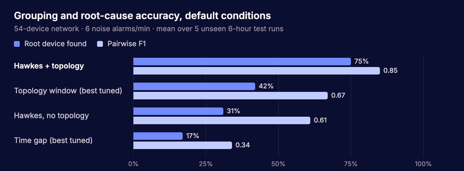
Figure 1. Root device found and pairwise F1 by method at default settings, mean of 5 unseen test runs.

54-device network, 6 noise alarms/min, 5 s clock skew, 15% alarm loss, ~4 incidents/hour.

Across conditions

The rules degrade quickly as background noise rises; the Hawkes model degrades slowly.

Figure 2. Pairwise F1 as background noise rises. The tuned rules collapse to 0.03 at 30 alarms/min; the Hawkes model holds 0.60.

"Rules" = best tuned topology-window method for that condition. Hawkes won on both measures in all 9 conditions.

What the model learned by itself

The fitted α matrix is readable. The strongest learned links were:

This is the cascade an experienced network engineer would draw on a whiteboard: optics degrade before the link drops, lost routing adjacencies take hosts and applications down with them. Nobody labelled any of it. For a NOC this matrix is useful on its own: it is an auditable, learned "what causes what" map for their network.

What it means

• The topology is what makes this work. Without it the same model dropped from 0.85 to 0.61 F1, and to 0.01 under heavy noise, because it merges unrelated alarms from across the network. The topology alone is not enough either: the rule engine has the same map and scores far lower. The gain comes from combining the map with learned timing and cause-effect strengths.

• Noise is where the difference shows most. Rules work by closeness in time and space, so every noisy alarm near an incident gets pulled in, and every noisy alarm on an upstream device can be mistaken for the root. The Hawkes model asks a better question: is this alarm more likely explained by a nearby alarm, or by the normal background rate for its type? Routine CPU spikes have a high background rate, so they rarely get blamed.

• Clock skew hurt less than expected. With tool clocks off by 60 seconds, root accuracy only dropped from 80% to 75%. The model learns links in both directions (for example host-unreachable ↔ app-timeout), which absorbs a consistent offset between tools.

• It is cheap. Fitting a day of alarms (13,638 events) takes 1.6 seconds, and grouping a 6-hour window (3,348 events) takes 0.04 seconds on one CPU core. It can run continuously.

• It also gives prediction for free. The same fitted rates estimate how an alarm that is happening now is likely to spread. We have not tested that here.

Limits

Read these before quoting any number.

• Synthetic data. Everything above is on a simulator. The simulator's timing is not Hawkes, but its structure (faults spread along the topology; alarm types have consistent causes) matches what the model assumes. Real networks will be messier. The next step is real alarm data with known root causes.

• Same author for simulator and model. This can bias results. An independent dataset, or someone else building the simulator, would remove it.

• The model still splits incidents. 1.8 tickets per incident is better than the rules (2.9), but not 1.0. Long outages sometimes get split when polling gaps exceed the slow decay.

• Parents must come first in time. If a downstream tool's clock runs ahead of the root device's, the true root can appear after its effects, and the model cannot link backwards. The skew tests suggest this is tolerable at up to 60 s, but it is a real limit.

• Small network. 54 devices. The method scales roughly with alarms × nearby alarms, so it should hold for thousands of devices, but we have not measured that.

Next steps

1. Run on real alarm streams with known root causes: a public telecom alarm dataset, or a customer's historical tickets.

2. Test cascade prediction: given the first 30 seconds of an incident, predict which devices will alarm next.

3. Scale test on a 5,000+ device topology.

4. Add a "reverse link" for known clock offsets between tools, so a root can still be found when it appears late.

References

A. G. Hawkes, Spectra of some self-exciting and mutually exciting point processes, Biometrika, 1971.

R. Cai et al., THP: Topological Hawkes Processes for learning causal structure on event sequences, IEEE TNNLS, 2022.